Pages

Wednesday 27 February 2019

Advantages and Disadvantages of Cross Validation in Machine Learning

Cross Validation in Machine Learning is a great technique to deal with overfitting problem in various algorithms. Instead of training our model on one training dataset, we train our model on many datasets. Below are some of the advantages and disadvantages of Cross Validation in Machine Learning:

Advantages of Cross Validation

1. Reduces Overfitting: In Cross Validation, we split the dataset into multiple folds and train the algorithm on different folds. This prevents our model from overfitting the training dataset. So, in this way, the model attains the generalization capabilities which is a good sign of a robust algorithm.

Note: Chances of overfitting are less if the dataset is large. So, Cross Validation may not be required at all in the situation where we have sufficient data available.

2. Hyperparameter Tuning: Cross Validation helps in finding the optimal value of hyperparameters to increase the efficiency of the algorithm.

More details...

Disadvantages of Cross Validation

1. Increases Training Time: Cross Validation drastically increases the training time. Earlier you had to train your model only on one training set, but with Cross Validation you have to train your model on multiple training sets. 

For example, if you go with 5 Fold Cross Validation, you need to do 5 rounds of training each on different 4/5 of available data. And this is for only one choice of hyperparameters. If you have multiple choice of parameters, then the training period will shoot too high.

2. Needs Expensive Computation: Cross Validation is computationally very expensive in terms of processing power required.

Tuesday 26 February 2019

What are Hyperparameters in Machine Learning Algorithms? How is Cross Validation used for Hyperparameter Tuning?

Hyperparameters are the parameters which we pass to the Machine Learning algorithms to maximize their performance and accuracy. 

For example, we need to pass the optimal value of K in the KNN algorithm so that it delivers good accuracy as well as does not underfit / overfit. Our model should have a good generalization capability. So, choosing the optimal value of the hyperparameter is very crucial in the Machine Learning algorithms.

Related: How to choose optimal value of K in KNN Algorithm? 

Examples of Hyperparameters

1. K in KNN (Number of nearest neighbors in KNN algorithm)

2. K in K-Means Clustering (Number of clusters in K-Means Clustering algorithm)

3. Depth of a Decision Tree

4. Number of Leaf Nodes in a Decision Tree

5. Number of Trees in a Random Forest

6. Step Size and Learning Rate in Gradient Descent (or Stochastic Gradient Descent)

7. Regularization Penalty (Lambda) in Ridge and Lasso Regression

Hyperparameters are also called "meta-parameters" and "free parameters".

Hyperparameters and Cross Validation

Selecting the optimal value of hyperparameters is usually not an easy task. These parameters are usually chosen using cross validation. These values remain fixed once chosen throughout the training of the model. 

In a K Fold Cross Validation, we initialize hyper-parameters to some value and and then train our model K times, every time using different Test Folds. Note down the average performance of the model over all the test folds and repeat the whole process for another set of hyper-parameters. Then we choose the set of hyper-parameters that corresponds to the best performance during cross-validation. 

As you can see, the computation cost of this process heavily depends on the number of hyper-parameter sets that need to be considered. 

Finding good hyper-parameters allows to avoid or at least reduce overfitting, but keep in mind that hyper-parameters can also overfit the data.

How to choose optimal value of K in KNN Algorithm?

There is no straightforward method to calculate the value of K in KNN. You have to play around with different values to choose the optimal value of K. Choosing a right value of K is a process called Hyperparameter Tuning.

The value of optimum K totally depends on the dataset that you are using. The best value of K for KNN is highly data-dependent. In different scenarios, the optimum K may vary. It is more or less hit and trail method.

You need to maintain a balance while choosing the value of K in KNN. K should not be too small or too large. 

A small value of K means that noise will have a higher influence on the result. 

Larger the value of K, higher is the accuracy. If K is too large, you are under-fitting your model. In this case, the error will go up again. So, at the same time you also need to prevent your model from under-fitting. Your model should retain generalization capabilities otherwise there are fair chances that your model may perform well in the training data but drastically fail in the real data. Larger K will also increase the computational expense of the algorithm.

There is no one proper method of estimation of K value in KNN. No method is the rule of thumb but you should try considering following suggestions:

1. Square Root Method: Take square root of the number of samples in the training dataset.

2. Cross Validation Method: We should also use cross validation to find out the optimal value of K in KNN. Start with K=1, run cross validation (5 to 10 fold),  measure the accuracy and keep repeating till the results become consistent. 

K=1, 2, 3... As K increases, the error usually goes down, then stabilizes, and then raises again. Pick the optimum K at the beginning of the stable zone. This is also called Elbow Method.

3. Domain Knowledge also plays a vital role while choosing the optimum value of K.

4. K should be an odd number.

I would suggest to try a mix of all the above points to reach any conclusion. 

Monday 25 February 2019

Which Machine Learning Algorithms require Feature Scaling (Standardization and Normalization) and which not?

Feature Scaling (Standardization and Normalization) is one of the important steps while preparing the data. Whether to use feature scaling or not depends upon the algorithm you are using. Some algorithms require feature scaling and some don't. Lets see it in detail.

Algorithms which require Feature Scaling (Standardization and Normalization)

Any machine learning algorithm that computes the distance between the data points needs Feature Scaling (Standardization and Normalization). This includes all curve based algorithms. 

Example:

1. KNN (K Nearest Neigbors)
2. SVM (Support Vector Machine)
3. Logistic Regression
4. K-Means Clustering

Algorithms that are used for matrix factorization, decomposition and dimensionality reduction also require feature scaling.

Example:

1. PCA (Principal Component Analysis)
2. SVD (Singular Value Decomposition)

Why is Feature Scaling required? 

Consider a dataset which contains the age and salary of the employee. Now age is a 2 digit number while salary would be of 5 to 6 digit. If we don't scale both the features (age and salary), salary will adversely affect the accuracy of the algorithm (if the algorithm is distance based). So, if we don't scale the features, then large scale features will dominate the small scale features due to which algorithm will produce wrong predictions.

Algorithms which don't require Feature Scaling (Standardization and Normalization)

The algorithms which rely on rules like tree based algorithms don't require Feature Scaling (Standardization and Normalization).

Example:

1. CART (Classification and Regression Trees)
2. Random Forests
3. Gradient Boosted Decision Trees

Algorithms that rely on distributions of the variables also don't need feature scaling.

Example: 

1. Naive Bayes 

Related Article: Why to standardize and transform the features in the dataset before applying Machine Learning algorithms?

Sunday 24 February 2019

Loss Functions in Machine Learning (MAE, MSE, RMSE)

Loss Function indicates the difference between the actual value and the predicted value. If the magnitude of the loss function is high, it means our algorithm is showing a lot of variance in the result and needs to be corrected. 

Lets look into the types of loss functions in Machine Learning in detail. There are broadly two types of losses based on the type of algorithm we are using:

Types of Losses:

1. Regression Losses
2. Classification Losses

Lets first discuss regression losses:

1. Mean Absolute Error (MAE) or (L1 Loss)
2. Mean Squared Error (MSE) or (Quadratic Loss) or (L2 Loss)
3. Root Mean Squared Error (RMSE)
4. Mean Bias Error

1. Mean Absolute Error (MAE) or (L1 Loss)

This is the average of the sum of absolute differences between predicted values and actual values.

2. Mean Squared Error (MSE) or (Quadratic Loss) or (L2 Loss)

This is the average of the sum of squared difference between predicted values and actual values.

3. Root Mean Squared Error (RMSE)

This is a square root of the MSE (L2)


4. Mean Bias Error

Just like MAE (L1), but we don't take absolute value here. So, there is a possibility of negative values cancelling out positive values. That is why it is not that much popular loss function. Although less accurate in practice, it could determine if the model has positive bias or negative bias.

Regression Loss Functions in Scikit Learn Library in Python

mean_absolute_error and mean_squared_error are present in sklearn.metrics. Just import them like this:

from sklearn.metrics import mean_absolute_error, mean_squared_error 

You can calculate loss function like below. Here "y_test" is the actual value and "y_pred" is the predicted value.

meanAbsoluteError = mean_absolute_error(y_test, y_pred)
meanSquaredError = mean_squared_error(y_test, y_pred)
rootMeanSquaredError = np.sqrt(meanSquaredError)

print('Mean Absolute Error:', meanAbsoluteError)  

print('Mean Squared Error:', meanSquaredError)  
print('Root Mean Squared Error:', rootMeanSquaredError)

I will write on classification losses later on. So, stay tuned.

Implement Multiple Linear Regression Algorithm in Python using Scikit Learn Library

Linear Regression model basically finds out the best value for the intercept and the slope, which results in a line that best fits the data. Linear Regression can be classified as Simple Linear Regression and Multiple Linear Regression

Linear Regression involving multiple variables is called Multiple Linear Regression. I implemented Simple Linear Regression in my previous article. In this article, we will implement Multiple Linear Regression. We will try to predict the petrol consumption in US.

You can download petrol_consumption.csv from here. You can also download my Jupyter notebook containing below code of Multiple Linear Regression.

Step 1: Import the required Python libraries like pandas, numpy and sklearn

import pandas as pd
import numpy as np
from sklearn.model_selection import train_test_split
from sklearn.linear_model import LinearRegression
from sklearn.metrics import mean_absolute_error, mean_squared_error 

Step 2: Load and examine the dataset

names = ['Index', 'One', 'Petrol tax (cents per gallon)', 'Average income (dollars)', 
                'Paved Highways (miles)', 'Proportion of population with driver licenses',
                'Consumption of petrol (millions of gallons)']

dataset = pd.read_csv('petrol_consumption.csv', names=names)

dataset.shape
dataset.head()
dataset.describe() 

Please note that "describe()" is used to display the statistical values of the data like mean and standard deviation.

I got mean of the Consumption of petrol (millions of gallons) as 576.770833. I will use this value to evaluate the performance of the algorithm in step 8.

Step 3: Mention X and Y axis

X = dataset[['Petrol tax (cents per gallon)', 'Average income (dollars)', 
                    'Paved Highways (miles)', 'Proportion of population with driver licenses']]

y = dataset['Consumption of petrol (millions of gallons)']

X contains the list of attributes
Y contains the list of labels

Step 4: Split the dataset into training and testing dataset

X_train, X_test, y_train, y_test = train_test_split(X, y, test_size = 0.20, random_state=0) 

Step 5: Create and fit the model

model = LinearRegression()
model.fit(X_train, y_train)  

Step 6: Print coefficient (slope) for all the features

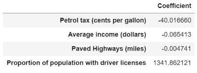
In case of multi-variable linear regression, the regression model has to find the most optimal coefficients for all the attributes. To see what coefficients our regression model has chosen, execute the following script:

coeff_df = pd.DataFrame(model.coef_, X.columns, columns=['Coefficient'])  
coeff_df  


We can use these coefficients (slopes) to find out which feature has the highest impact on the predicted output and how different features relate to each other.

This means that for a unit increase in "Petrol Tax", there is a decrease of 40.01 million gallons in gas consumption. Similarly, a unit increase in proportion of population with a drivers license results in an increase of 1.341 billion gallons of gas consumption. We can see that "Average income" and "Paved Highways" have a very little effect on the gas consumption.

Step 7: Predict from the model

y_pred = model.predict(X_test)

The y_pred is a numpy array that contains all the predicted values for the input values in the X_test.

Lets see the difference between the actual and predicted values.

df=pd.DataFrame({'Actual':y_test, 'Predicted':y_pred})  
df 

Step 8: Check the accuracy

meanAbsoluteError = mean_absolute_error(y_test, y_pred)
meanSquaredError = mean_squared_error(y_test, y_pred)
rootMeanSquaredError = np.sqrt(meanSquaredError)
print('Mean Absolute Error:', meanAbsoluteError)  
print('Mean Squared Error:', meanSquaredError)  
print('Root Mean Squared Error:', rootMeanSquaredError)

I got Root Mean Square Error as 68.31064915215168 which is slightly higher than 10% of the mean value of the Consumption of petrol (millions of gallons) i.e. 576.770833 (look at step 2). This means that our algorithm needs improvement, but even then it did a decent job.

We can improve the performance of the algorithm by considering below points:

1. Gather more data: More the data, more the accuracy.

2. Visualizing the data: We made the assumption that this data has a linear relationship, but that might not be the case. Visualizing the data may help you determine that.

3. Hyperparameter Tuning: Use cross-validation and try different combinations of sub-sets and hyperparameters to gain accuracy.

4. Feature Extraction: We don't have sufficient features to accurately predict the petrol consumption. We should also use feature elimination and extraction techniques (dimensionality reduction techniques like PCA, MDS, LDA etc). We should eliminate the variables which have high correlation.

Implement Simple Linear Regression Algorithm in Python using Scikit Learn Library

Linear Regression model basically finds out the best value for the intercept and the slope, which results in a line that best fits the data. Linear Regression can be classified as Simple Linear Regression and Multiple Linear Regression

Simple Linear Regression involves only two variables. One is Attribute and another is Label. Attributes are the independent variables while labels are the dependent variables whose values are to be predicted. 

In this article, we will implement Simple Linear Regression. Lets predict the percentage of marks that a student is expected to score based upon the number of hours he studied. This is a simple linear regression task as it involves just two variables. "Hours Studied" is an independent variable (attribute) and "Percentage Scored" is a dependent variable (label) which we are going to predict using Simple Linear Regression.

You can download student_scores.csv from here. You can also download my Jupyter notebook containing below code of Simple Linear Regression.

Step 1: Import the required Python libraries like pandas, numpy and sklearn

import pandas as pd
import numpy as np
import matplotlib.pyplot as plt  
%matplotlib inline
from sklearn.model_selection import train_test_split
from sklearn.linear_model import LinearRegression
from sklearn.metrics import mean_absolute_error, mean_squared_error 

Step 2: Load and examine the dataset

dataset = pd.read_csv('student_scores.csv') 
dataset.shape
dataset.head()
dataset.describe() 

Please note that "describe()" is used to display the statistical values of the data like mean and standard deviation.

I got mean of the scores as 51.480000. I will use this value to evaluate the performance of the algorithm in step 9.

Step 3: Draw a plot between attribute and label

dataset.plot(x='Hours', y='Scores', style='o')  
plt.title('Hours vs Percentage')  
plt.xlabel('Hours Studied')  
plt.ylabel('Percentage Score')  
plt.show() 

The plot will show a positive linear relation between the number of hours studied and percentage of score.

Step 4: Mention X and Y axis

X = dataset.iloc[:, :-1].values  
y = dataset.iloc[:, 1].values  

X contains the list of attributes
Y contains the list of labels

Step 5: Split the dataset into training and test dataset

X_train, X_test, y_train, y_test = train_test_split(X, y, test_size = 0.20, random_state=0) 

Step 6: Create and fit the model

model = LinearRegression()
model.fit(X_train, y_train)  

Step 7: Print intercept and coefficient (slope) of the best fit line

print(model.intercept_) 
print(model.coef_)  

I get the intercept as 2.018160041434683 and coefficient as 9.91065648. This means that for every one unit of change in hours studied, the change in the score is about 9.91%. Or in simpler words, if a student studies one hour more than he previously studied for an exam, he can expect to achieve an increase of 9.91% in the score.

Step 8: Predict from the model

y_pred = model.predict(X_test)

The y_pred is a numpy array that contains all the predicted values for the input values in the X_test.

Lets see the difference between the actual and predicted values.

df=pd.DataFrame({'Actual':y_test, 'Predicted':y_pred})  
df 

Step 9: Check the accuracy

meanAbsoluteError = mean_absolute_error(y_test, y_pred)
meanSquaredError = mean_squared_error(y_test, y_pred)
rootMeanSquaredError = np.sqrt(meanSquaredError)
print('Mean Absolute Error:', meanAbsoluteError)  
print('Mean Squared Error:', meanSquaredError)  
print('Root Mean Squared Error:', rootMeanSquaredError)

I got Root Mean Square Error as 4.6474476121003665 which is less than 10% of the mean value of the percentages of all the students i.e. 51.48 (look at step 2). This means that our algorithm did a decent job.

Advantages and Disadvantages of Decision Trees in Machine Learning

Decision Tree is used to solve both classification and regression problems. But the main drawback of Decision Tree is that it generally leads to overfitting of the data. Lets discuss its advantages and disadvantages in detail.

Advantages of Decision Tree

1. Clear VisualizationThe algorithm is simple to understand, interpret and visualize as the idea is mostly used in our daily lives. Output of a Decision Tree can be easily interpreted by humans.

2. Simple and easy to understand: Decision Tree looks like simple if-else statements which are very easy to understand.

3. Decision Tree can be used for both classification and regression problems.

4. Decision Tree can handle both continuous and categorical variables.

5. No feature scaling required: No feature scaling (standardization and normalization) required in case of Decision Tree as it uses rule based approach instead of distance calculation.

6. Handles non-linear parameters efficiently: Non linear parameters don't affect the performance of a Decision Tree unlike curve based algorithms. So, if there is high non-linearity between the independent variables, Decision Trees may outperform as compared to other curve based algorithms.

7. Decision Tree can automatically handle missing values.

8. Decision Tree is usually robust to outliers and can handle them automatically.

9. Less Training Period: Training period is less as compared to Random Forest because it generates only one tree unlike forest of trees in the Random Forest. 

Disadvantages of Decision Tree

1. Overfitting: This is the main problem of the Decision Tree. It generally leads to overfitting of the data which ultimately leads to wrong predictions. In order to fit the data (even noisy data), it keeps generating new nodes and ultimately the tree becomes too complex to interpret. In this way, it loses its generalization capabilities. It performs very well on the trained data but starts making a lot of mistakes on the unseen data.

I have written a detailed article on Overfitting here.

2. High variance: As mentioned in point 1, Decision Tree generally leads to the overfitting of data. Due to the overfitting, there are very high chances of high variance in the output which leads to many errors in the final estimation and shows high inaccuracy in the results. In order to achieve zero bias (overfitting), it leads to high variance. 

3. Unstable: Adding a new data point can lead to re-generation of the overall tree and all nodes need to be recalculated and recreated. 

4. Affected by noise: Little bit of noise can make it unstable which leads to wrong predictions.

5. Not suitable for large datasets: If data size is large, then one single tree may grow complex and lead to overfitting. So in this case, we should use Random Forest instead of a single Decision Tree.

In order to overcome the limitations of the Decision Tree, we should use Random Forest which does not rely on a single tree. It creates a forest of trees and takes the decision based on the vote count. Random Forest is based on bagging method which is one of the Ensemble Learning techniques.

Saturday 23 February 2019

Advantages and Disadvantages of KNN Algorithm in Machine Learning

KNN is a very simple algorithm used to solve classification problems. KNN stands for K-Nearest Neighbors. K is the number of neighbors in KNN. Lets find out some advantages and disadvantages of KNN algorithm.

Advantages of KNN

1. No Training Period: KNN is called Lazy Learner (Instance based learning). It does not learn anything in the training period. It does not derive any discriminative function from the training data. In other words, there is no training period for it. It stores the training dataset and learns from it only at the time of making real time predictions. This makes the KNN algorithm much faster than other algorithms that require training e.g. SVM, Linear Regression etc.

2. Since the KNN algorithm requires no training before making predictions, new data can be added seamlessly which will not impact the accuracy of the algorithm.

3. KNN is very easy to implement. There are only two parameters required to implement KNN i.e. the value of K and the distance function (e.g. Euclidean or Manhattan etc.)

Disadvantages of KNN

1. Does not work well with large dataset: In large datasets, the cost of calculating the distance between the new point and each existing points is huge which degrades the performance of the algorithm.

2. Does not work well with high dimensions: The KNN algorithm doesn't work well with high dimensional data because with large number of dimensions, it becomes difficult for the algorithm to calculate the distance in each dimension.

3. Need feature scaling: We need to do feature scaling (standardization and normalization) before applying KNN algorithm to any dataset. If we don't do so, KNN may generate wrong predictions.

4. Sensitive to noisy data, missing values and outliers: KNN is sensitive to noise in the dataset. We need to manually impute missing values and remove outliers.

Advantages and Disadvantages of Random Forest Algorithm in Machine Learning

Random Forest is a powerful algorithm in Machine Learning. It is based on the Ensemble Learning technique (bagging). Following are the advantages and disadvantages of Random Forest algorithm.

Advantages of Random Forest

1. Random Forest is based on the bagging algorithm and uses Ensemble Learning technique. It creates as many trees on the subset of the data and combines the output of all the trees. In this way it reduces overfitting problem in decision trees and also reduces the variance and therefore improves the accuracy.

2. Random Forest can be used to solve both classification as well as regression problems.

3. Random Forest works well with both categorical and continuous variables.

4. Random Forest can automatically handle missing values.

5. No feature scaling required: No feature scaling (standardization and normalization) required in case of Random Forest as it uses rule based approach instead of distance calculation.

6. Handles non-linear parameters efficiently: Non linear parameters don't affect the performance of a Random Forest unlike curve based algorithms. So, if there is high non-linearity between the independent variables, Random Forest may outperform as compared to other curve based algorithms.

7. Random Forest can automatically handle missing values.

8. Random Forest is usually robust to outliers and can handle them automatically.

9. Random Forest algorithm is very stable. Even if a new data point is introduced in the dataset, the overall algorithm is not affected much since the new data may impact one tree, but it is very hard for it to impact all the trees.

10. Random Forest is comparatively less impacted by noise.

Disadvantages of Random Forest

1. Complexity: Random Forest creates a lot of trees (unlike only one tree in case of decision tree) and combines their outputs. By default, it creates 100 trees in Python sklearn library. To do so, this algorithm requires much more computational power and resources. On the other hand decision tree is simple and does not require so much computational resources.

2. Longer Training Period: Random Forest require much more time to train as compared to decision trees as it generates a lot of trees (instead of one tree in case of decision tree) and makes decision on the majority of votes.

Implement Random Forest Algorithm in Python using Scikit Learn Library for Regression Problem

Random Forest is a bagging algorithm based on Ensemble Learning technique. The Random Forest algorithm can be used for both classification and regression problems. 

In last article, we had solved a classification problem using Random Forest. In this article, we will solve a regression problem (predicting the petrol consumption in US) using Random Forest. We need to import RandomForestRegressor instead of RandomForestClassifier from sklearn library to implement Random Forest.

To measure the performance of a regression problem, we need to import mean_absolute_error and mean_squared_error metrics instead of confusion_matrix, accuracy_score and classification_report which we used in classification problem.

You can download petrol_consumption.csv from here. You can also download my Jupyter notebook containing below code of Random Forest implementation.

Step 1: Import the required Python libraries like pandas, numpy and sklearn

import pandas as pd
import numpy as np
from sklearn.preprocessing import StandardScaler
from sklearn.model_selection import train_test_split
from sklearn.ensemble import RandomForestRegressor
from sklearn.metrics import mean_absolute_error, mean_squared_error 

Step 2: Load and examine the dataset

names = ['Index', 'One', 'Petrol tax (cents per gallon)', 'Average income (dollars)', 
                'Paved Highways (miles)', 'Proportion of population with driver licenses',
                'Consumption of petrol (millions of gallons)']

dataset = pd.read_csv('petrol_consumption.csv', names=names)

dataset.shape
dataset.head()
dataset.describe() 

Please note that "describe()" is used to display the statistical values of the data like mean and standard deviation.

Step 3: Mention X and Y axis

X = dataset.iloc[:, 2:6].values
y = dataset.iloc[:, 6].values 

Please note that first two columns "Index" and "One" are of no use for making any prediction. So excluded these two features. Also excluded the label which is the last column.

X contains the list of attributes
Y contains the list of labels

Step 4: Split the dataset into training and testing dataset

X_train, X_test, y_train, y_test = train_test_split(X, y, test_size = 0.20, random_state=0) 

Step 5: Scale the features

standardScaler = StandardScaler()  
X_train = standardScaler.fit_transform(X_train)
X_test = standardScaler.transform(X_test) 

This step is not must for Random Forest as it is being taken care by Random Forest internally. Feature scaling is not required in tree based algorithms.

Step 6: Create and fit the model

model = RandomForestRegressor(n_estimators=120, random_state=0) 
model.fit(X_train, y_train)  

"n_estimators" is the number of trees we want to create in a Random Forest. By default, it is 100.

Step 7: Predict from the model

y_pred = model.predict(X_test)

The y_pred is a numpy array that contains all the predicted values for the input values in the X_test.

Lets see the difference between the actual and predicted values.

df=pd.DataFrame({'Actual':y_test, 'Predicted':y_pred})  
df 

Step 8: Check the accuracy

meanAbsoluteError = mean_absolute_error(y_test, y_pred)
meanSquaredError = mean_squared_error(y_test, y_pred)
rootMeanSquaredError = np.sqrt(meanSquaredError)
print('Mean Absolute Error:', meanAbsoluteError)  
print('Mean Squared Error:', meanSquaredError)  
print('Root Mean Squared Error:', rootMeanSquaredError)

Implement Random Forest Algorithm in Python using Scikit Learn Library for Classification Problem

Random Forest is a bagging algorithm based on Ensemble Learning technique. The random forest algorithm can be used for both classification and regression problems. 

In this article, we will solve a classification problem (bank note authentication) using Random Forest. We need to import RandomForestClassifier from sklearn library to implement Random Forest.

You can download bank_note_authentication.csv from here. You can also download my Jupyter notebook containing below code of Random Forest implementation.

Step 1: Import the required Python libraries like pandas and sklearn

import pandas as pd
from sklearn.preprocessing import StandardScaler
from sklearn.model_selection import train_test_split
from sklearn.ensemble import RandomForestClassifier
from sklearn.metrics import confusion_matrix, accuracy_score, classification_report

Step 2: Load and examine the dataset

names = ['Variance', 'Skewness', 'Curtosis', 'Entropy', 'Class']
dataset = pd.read_csv('bank_note_authentication.csv', names=names)
dataset.shape
dataset.head()

Step 3: Mention X and Y axis

X = dataset.iloc[:, 0:4].values  
y = dataset.iloc[:, 4].values 

Step 4: Split the dataset into training and testing dataset

X_train, X_test, y_train, y_test = train_test_split(X, y, test_size = 0.20) 

Step 5: Scale the features

standardScaler = StandardScaler()  
X_train = standardScaler.fit_transform(X_train)  
X_test = standardScaler.transform(X_test) 

This step is not must for Random Forest as it is being taken care by Random Forest internally. Feature scaling is not required in tree based algorithms.

Step 6: Create and fit the model

model =  RandomForestClassifier(n_estimators=20, random_state=0) 
model.fit(X_train, y_train)  

"n_estimators" is the number of trees we want to create in a Random Forest. By default, it is 100.

Step 7: Predict from the model

y_pred = model.predict(X_test)

The y_pred is a numpy array that contains all the predicted values for the input values in the X_test.

Lets see the difference between the actual and predicted values.

df = pd.DataFrame({'Actual': y_test, 'Predicted': y_pred})  
df  

Step 8: Check the accuracy

confusionMatrix = confusion_matrix(y_test, y_pred)
accuracyScore = accuracy_score(y_test, y_pred)
classificationReport = classification_report(y_test, y_pred)
print(confusionMatrix)
print(accuracyScore * 100)
print(classificationReport)

Friday 22 February 2019

Implement Decision Tree Algorithm in Python using Scikit Learn Library for Regression Problem

Lets implement Decision Tree algorithm in Python using Scikit Learn library. In my last article, we had solved a classification problem using Decision Tree. This time, we will solve a regression problem (predicting the petrol consumption in US) using Decision Tree.

We need to import DecisionTreeRegressor from sklearn library instead of DecisionTreeClassifier to implement Decision Tree to solve regression problem. 

To measure the performance of a regression problem, we need to import mean_absolute_error and mean_squared_error metrics instead of confusion_matrix, accuracy_score and classification_report which we used in classification problem.

You can download petrol_consumption.csv from here. You can also download my Jupyter notebook containing below code of Decision Tree implementation.

Step 1: Import the required Python libraries like pandas, numpy and sklearn

import pandas as pd
import numpy as np
from sklearn.model_selection import train_test_split
from sklearn.tree import DecisionTreeRegressor
from sklearn.metrics import mean_absolute_error, mean_squared_error 

Step 2: Load and examine the dataset

names = ['Index', 'One', 'Petrol tax (cents per gallon)', 'Average income (dollars)', 
                'Paved Highways (miles)', 'Proportion of population with driver licenses',
                'Consumption of petrol (millions of gallons)']

dataset = pd.read_csv('petrol_consumption.csv', names=names)

dataset.shape
dataset.head()
dataset.describe() 

Please note that "describe()" is used to display the statistical values of the data like mean and standard deviation.

Step 3: Mention X and Y axis

X = dataset.drop('Index', axis=1).drop('One', axis=1).drop('Consumption of petrol (millions of gallons)', axis=1)  

Please note that first two columns "Index" and "One" are of no use for making any prediction. So dropped these two features. Also dropped the label which is the last column.

X contains the list of attributes
Y contains the list of labels

y = dataset['Consumption of petrol (millions of gallons)']  

X.head()
y.head()

Step 4: Split the dataset into training and testing dataset

X_train, X_test, y_train, y_test = train_test_split(X, y, test_size = 0.20, random_state=0) 

Step 5: Create and fit the model

model = DecisionTreeRegressor() 
model.fit(X_train, y_train)  

Step 6: Predict from the model

y_pred = model.predict(X_test)

The y_pred is a numpy array that contains all the predicted values for the input values in the X_test.

Lets see the difference between the actual and predicted values.

df=pd.DataFrame({'Actual':y_test, 'Predicted':y_pred})  
df 

Step 7: Check the accuracy

meanAbsoluteError = mean_absolute_error(y_test, y_pred)
meanSquaredError = mean_squared_error(y_test, y_pred)
rootMeanSquaredError = np.sqrt(meanSquaredError)
print('Mean Absolute Error:', meanAbsoluteError)  
print('Mean Squared Error:', meanSquaredError)  
print('Root Mean Squared Error:', rootMeanSquaredError)

About the Author

I have more than 10 years of experience in IT industry. Linkedin Profile

I am currently messing up with neural networks in deep learning. I am learning Python, TensorFlow and Keras.

Author: I am an author of a book on deep learning.

Quiz: I run an online quiz on machine learning and deep learning.