Pages

Friday 31 May 2019

Activation (Squashing) Functions in Deep Learning: Step, Sigmoid, Tanh and ReLu

There are mainly four activation functions (step, sigmoid, tanh and relu) used in neural networks in deep learning. These are also called squashing functions as these functions squash the output under certain range. We will also see various advantages and disadvantages of different activation functions. 

Importance of Activation Functions in Neural Networks

These activation functions help in achieving non-linearity in deep learning models. If we don't use these non-linear activation functions, neural network would not be able to solve the complex real life problems like image, video, audio, voice and text processing, natural language processing etc. because our neural network would still be linear and linear models cannot solve real life complex problems. 

Although linear models are simple but are computationally weak and not able to handle complex problems. So, if you don't use activation functions, no matter how many hidden layers you use in your neural network, it will still be linear an inefficient.

Lets discuss these activation functions in detail.

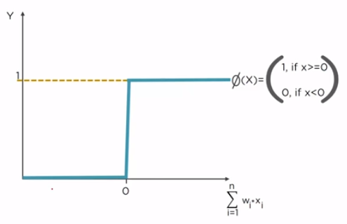
1. Step (Threshold) Activation Function

It either outputs 0 or 1 (Yes or No). It is non-linear in nature.


There is a sudden change in the decision (from 0 to 1) when input value crosses the threshold value. For most real-world applications, we would expect a smoother decision function which gradually changes from 0 to 1.

Lets take a real life example of this step function. Consider a movie. If the critics rating is below or equal to 0.5, step function will output 0 (don't watch this movie). If it is above 0.50, step function will output 1 (go and watch this movie). 

What would be the decision for a movie with critics rating = 0.51? Yes!
What would be the decision for a movie with critics rating = 0.49? No!

It appears harsh that we would watch a movie with a rating of 0.51 but not the one with a rating of 0.49 and this is where sigmoid function comes into the picture. 

As step function either outputs 0 or 1 (Yes or No), it is a non-differentiable activation function and therefore its derivative will always be zero. 

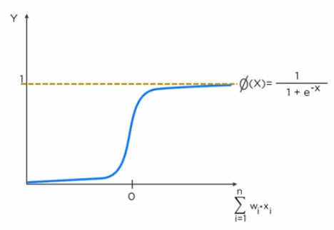
2. Sigmoid Activation Function

It is also called Logistic activation function. Its output ranges from 0 to 1. It has "S" shaped curve. Sigmoid function is much smoother than the step function which seems logical and obvious in real life example as discussed above.


Advantages of Sigmoid Activation Function

1. Sigmoid is a non-linear activation function.

2. Instead of just outputting 0 and 1, it can output any value between 0 and 1 like 0.62, 0.85, 0.98 etc. So, instead of just Yes or No, it outputs a probability value. So, the output of sigmoid function is is smooth, continuous and differentiable

3. As the range of output remains between 0 and 1, it cannot blow up the activations unlike ReLu activation function.

Disadvantages of Sigmoid Activation Function

1. Vanishing and exploding gradients problem

2. Computing the exponential may be expensive sometimes

3. Tanh (Hyperbolic Tangent) Activation Function

It is similar to Sigmoid Activation Function, the only difference is that it outputs the values in the range of -1 to 1 instead of 0 and 1 (like sigmoid function). So, we can say that tanh function is zero centered (unlike sigmoid function) as its values range from -1 to 1 instead of 0 to 1.


Advantages and Disadvantages of Tanh activation function are same as that of sigmoid activation function.

4. ReLu (Rectified Linear Unit)

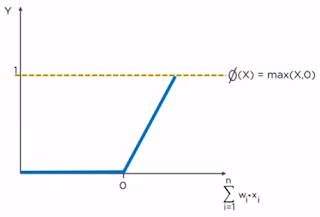
ReLU outperforms both sigmoid and tanh functions and is computationally more efficient compared to both. Given an input value, the ReLu will generate 0, if the input is less than 0, otherwise the output will be the same as the input. 

Mathematically, relu(z) = max(0, z)


Advantages of ReLu Activation Function

1. It does not require exponent calculation as it is done in sigmoid and tanh activation functions.

2. It does not encounter vanishing gradient problem.

Disadvantages of ReLu

1. Dying ReLu: The dying ReLu is a phenomenon where a neuron in the network is permanently dead due to inability to fire in the forward pass. This problem occurs when the activation value generated by a neuron is zero while in forward pass, which resulting that its weights will get zero gradient. As a result, when we do back-propagation, the weights of that neuron will never be updated and that particular neuron will never be activated.

Leaky ReLU with a small positive gradient for negative inputs (y=0.01x when x < 0 say) is one attempt to address this issue and give a chance to recover. One more attempt is Max ReLU. I will add more details about these later on or may write a separate article.

2. Unbounded output range: Unbounded output values generated by ReLu could make the computation within the RNN likely to blow up to infinity without reasonable weights. As a result, the learning can be remarkably unstable because a slight shift in the weights in the wrong direction during back-propagation can blow up the activations during the forward pass.

Which one to use: We should use ReLu instead of sigmoid and tanh because of its high efficiency. ReLu should be used for hidden layers and softmax should be used for output layers for classification and regression problems.

A comparison between Machine Learning and Deep Learning (Machine Learning vs Deep Learning)

Deep Learning is considered as subset of Machine Learning. Both have a lot of similarities and differences. Lets compare Machine Learning and Deep Learning and see some of the differences between them.

1. Scale of data: Deep Learning algorithms work efficiently on high amount of data (both structured and unstructured). If there is less amount of data, deep learning algorithms may not perform well as compared to machine learning algorithms. Deep learning algorithms are best suited for unstructured data like images, videos, voice, natural language processing etc. Machine Learning algorithms are not capable of dealing with unstructured data.

2. Scale of computation: Deep Learning algorithms require high computational power. Deep Learning algorithms need high-end machines like GPUs as these heavily perform complex operations like matrix multiplications.

3. Feature Extraction: In machine learning, we need to manually identify the features from the dataset based on the domain knowledge and expertise. This takes a huge amount of time and effort. Also, there are a lot of chances that we can miss some of the important features which are crucial for prediction. 

For example, while image processing in machine learning, you need to extract the feature manually in the image like the eyes, nose, lips, pixel values, shape, textures, position, orientation and so on. Those extracted features are then fed to the machine learning model. The performance of most of the machine learning algorithms depends on how accurately the features are identified and extracted.

Deep learning solves this issue automatically using convoluted layers in CNN. The first layer of a neural network will learn small details from the picture like edges, lines etc; the next layers will combine the previous knowledge to make more complex information. 

4. Training Data: Deep Learning algorithms usually require more training data as compared to machine learning algorithms.

5. Data Augmentation: Creating new data by making reasonable modifications to the existing data is called data augmentation. Lets take an example of our MNIST dataset (hand written digits). We can easily generate thousands of new similar images by rotating, flipping, scaling, shifting, zooming in and out, cropping, changing or varying the color of the existing images. 

We can use data augmentation technique when our model is overfitting due to less data.

In many cases in deep learning, increasing the amount of data is not a difficult task as we discussed above the case of MNIST dataset. In machine learning, this task is not that easy as we need labelled data which is not easily available. 

6. Training Time: Deep Learning algorithms usually take a longer time to train as compared to machine learning algorithms as there are a lot of computations involved inside the hidden layers.

7. Testing Time: Deep Learning algorithms take much less testing time as compared to machine learning algorithms. 

8. Interpretability: Machine Learning algorithms are more interpretable as compared to deep learning algorithms. Deep learning models mostly act as black box.

For example, decision tree in machine learning can be easily interpreted by human beings and they can easily get to know how the final values are computed. On the other hand, it is very hard to know what calculations happened inside the hidden layers of neural networks, how convoluted layers in CNN identified the various portions of the images etc.

Let’s take another example. Suppose we use deep learning to give automated scoring to essays. The performance it gives in scoring is quite excellent and is near human performance. But there’s is an issue. It does not reveal why it has given that score. Indeed mathematically you can find out which nodes of a deep neural network were activated, but we don’t know what there neurons were supposed to model and what these layers of neurons were doing collectively. So we fail to interpret the results.

9. Dimensionality: As the dimension of the data increases, efficiency of machine learning algorithms starts degrading. Although we have some dimensionality reduction techniques in machine learning like PCA, t-SNE, SVD, MDS etc but deep learning takes care of dimensionality very well. 

10. Computer Vision: Deep Learning algorithms help in solving a lot of computer vision problems like:

A) Image Classification
B) Image Classification With Localization
C) Object Detection
D) Object Segmentation
E) Image Style Transfer
F) Image Colorization
G) Image Reconstruction
H) Image Super-Resolution
I) Image Synthesis

For more details on computer vision, please visit this article.

Machine Learning algorithms have limited capacity and efficiency in resolving these computer vision problems while convolutional neural networks are very efficient in handling these tasks.

Thursday 30 May 2019

A journey from a simple Perceptron (Artificial Neuron) to complex Neural Networks

Perceptron is an artificial neuron and is the fundamental unit of a neural network in deep learning. It is also called single layer neural network or single layer binary linear classifier.

Perceptron takes inputs which can be real or boolean, assigns random weights to the inputs along with a bias, takes their weighted sum, pass it through a threshold function which will decide whether to take any action on it or not depending upon some threshold value, and finally perform linear binary classifications. This threshold function is usually a step function.

Mathematical representation of perceptron looks like an if-else condition, if the weighted sum of the inputs is greater than a threshold value, output will be 1 else output will be 0.

Weights

Accuracy of an algorithm mainly depends upon the right assignment of the weights. That is what Gradient Descent does during back-propagation. 

Lets understand weights in layman language:

Consider a movie. Whether a person will go to see a movie or not depends upon different factors (features) like genre (comedy, horror, romance etc.), actor, director etc. Some people will give more weight to the genre and lesser weight to actor and director. Some will give more weight to the actor in the movie and lesser weight to genre.

Consider a cell phone. Generally, the relationship between the price of a phone and likeliness to buy a phone is inversely proportional (except for a few fan boys). For someone who is an iPhone fan, he/she will be more likely to buy a next version of the phone irrespective of its price. But on the other hand, an ordinary consumer may give more importance to budget offerings from other brands. 

The point here is, all the inputs don’t have equal importance in the decision making and weights for these features depend on the data and the task at hand.

Applications of Perceptrons

Perceptrons can be used to solve any problem which contains linearly separable set of inputs. For example, we can implement logic gates like OR and AND because these are linearly separable.

Limitation of Perceptrons

Perceptron can only learn linearly separable functions. It cannot handle non-linear inputs. For example, it cannot implement XOR gate as it can’t be classified by a linear separator. 

Neural Network

To address above limitation of Perceptrons, we’ll need to use a multi-layer perceptron, also known as feed-forward neural network. A neural network is a composition of perceptrons, connected in different ways and operating on different activation functions.

1. All the layers (input layer, hidden layers and output layer) are interconnected.

2. Weight is added to each input and then bias is added to per neuron and then it is passed to the activation function.

3. First forward propagate the weighted sum, calculate the error, backward propagate and update the weights using gradient descent and keep doing the same until a satisfactory result is achieved

Types of Neural Networks

1. Feed Forward Neural Network: This is the simplest neural network. Data flows only in forward direction from input layer to hidden layers to output layer. It may or may not have a hidden layer. At most it contains only one hidden layer. All nodes are fully connected. Back propagation method is used to train these kind of networks.

2. Deep Feed Forward Neural Network: Same as Feed Forward Neural Network. Difference is that, it has a lot more hidden layers. Back propagation method is used to train these kind of networks.

3. Radial Basis Function Neural Network: RBF neural networks are a type of feed forward neural networks that use radial basis function as activation function instead of logistic function. Instead of just outputting 0 or 1 (as in logistic function), radial basis functions consider the distance of a point with respect to the center.

4. CNN (Convolutional Neural Network)

5. Capsule Neural Networks

6. RNN (Recurrent Neural Network)

7. LSTM (Long Short-Term Memory Networks)

8. Autoencoders

For more types of neural networks, please visit this article.

Hidden Layers

The hidden layer is where the network stores it’s internal abstract representation of the training data, similar to the way that a human brain has an internal representation of the real world. 

Feature extraction happens at hidden layers. We can keep increasing the number of hidden layers to obtain higher accuracy. It should also be noted that increasing the number of layers above a certain point may lead the model to overfit.

Comparison of Deep and Shallow Neural Networks

Shallow neural networks have only one hidden layer as opposed to deep neural networks which have several hidden layers.

Advantages of Deep Neural Networks

1. Deep neural networks are better in learning and extracting features at various levels of abstraction as compared to shallow neural networks.

2. Deep neural networks have better generalization capabilities.

Disadvantages of Deep Neural Networks

1. Vanishing Gradients: As we add more and more hidden layers, back-propagation becomes less and less useful in passing information to the lower layers. As information is passed back, the gradients begin to vanish and become small relative to the weights of the networks.

2. Overfitting: As we keep on adding more and more layers to a neural network, chances of overfitting increase. So, we should maintain reasonable number of hidden layers in deep neural networks. 

3. Computational ComplexityAs we keep on adding more and more layers to a neural network, computational complexity increases. So, again, we should maintain reasonable number of hidden layers in deep neural networks. 

Activation Functions

Activation functions (like Sigmoid, Hyperbolic Tangent, Threshold, ReLuare what make a neural network adapt the non-linear behavior otherwise they will still be linear. For more details on activation functions, you can look into my this post.

Training Perceptrons using Back Propagation

The most common deep learning algorithm for supervised training of the multi-layer perceptrons is known as back-propagation. Following are the basic steps:

1. A training sample is presented and propagated forward through the network.

2. The output error is calculated, typically the mean squared error or root mean square error.

3. Weights are updated using Gradient Descent algorithm.

4. Above steps are repeated again and again until a satisfied result or accuracy is obtained.

Tuesday 28 May 2019

Basic introduction of various layers in CNN (Convolutional Neural Network)

CNN (Convolutional Neural Network) is a feed-forward neural network as the information moves from one layer to the next. CNN is also called ConvNet. It consists of hidden layers having convolution and pooling functions in addition to the activation function for introducing non-linearity. 

CNN is mainly used for image recognition. CNN first learns to recognize the components of an image (e.g. lines, corners, curves, shapes, texture etc.) and then learns to combine these components (pooling) to recognize larger structures (e.g. faces, objects etc.).

Layers in CNN

1. Convolutional Layer
2. ReLU Layer
3. Pooling Layer
4. Normalization Layer
5. Fully connected Layer

Computers see an input image as an array of pixels. Numerical representation of the pixels is processed through many layers of a CNN. Each input image passes through a series of hidden layers like convolutional layers with filters (kernals), ReLU layers, pooling layers and fully connected layers. These hidden layers perform feature extraction from the image.

Convolutional Layer

Convolution is the first layer to extract features from an input image. This layer uses a matrix filter and performs convolution operation to detect patterns in the image. Convolution of an image with different filters can perform operations such as edge detection, blur and sharpen by applying filters. 

Convolution is a mathematical operation that happens between two matrices (image matrix and a filter or kernal) to form a third matrix as an output (convoluted matrix). This output is also called feature map matrix.

Filters (Kernels): Filters act as pattern detectors. Filters help in finding out edges, curves, corners, textures, colors, dark and light areas in the image and many other details like height, width, and depth etc. Kernels keep sliding over an entire image to extract different components or patterns of an image. First filters learn to extract simple features in initial convoluted layers, and later on these filters get more sophisticated in deeper layers and find out complex patterns. 

We rotate this filter over an input matrix and get an output which is of less dimension.


Formula: Consider that our input matrix dimension is n X n. Filter size is f X f. Then our output matrix would be (n - f + 1) X (n - f + 1). Just replace n with 4, f with 3 and observe that the output matrix comes out to be 2 X 2.

Padding: We can observe that the input size is reduced from 4 X 4 to 2 X 2 after one convolution using 3 X 3 filter. This may lead to a problem. We may lose some information about edges and corners in the image. So, in order to preserve this information, we should use padding. 

Type of PaddingWe have two types of padding: Zero Padding and Valid Padding (no padding).

1. Zero Padding: Pad the image with zeros so that we don't lose any information about edges and corners.


In the above image, we have padded the input with zero. Now, if we use 3 X 3 filter over this, we get 4 X 4 output matrix (no reduction in dimensions) instead of 2 X 2.

2. Valid Padding: Drop the part of the image where the filter does not fit. This is called valid padding which keeps only valid part of the image. In this case, we compromise to lose some edge information in the image. We will get only 2 X 2 matrix in above example. We can go with this approach if we know that the information at edges is not that much useful and we can safely ignore that.

ReLU Layer

ReLU stands for Rectified Linear Unit for a non-linear operation. The output is Æ’(x) = max(0,x). ReLU’s main purpose is to introduce non-linearity in the ConvNet. It performs element-wise operation and set negative pixels to zero. 

ReLU function is applied to the output matrix (feature map matrix) in the convolutional layer and converts it into a rectified feature map matrix.

We can also use other activation functions like tanh and sigmoid but generally ReLU performs better than other activation functions in many scenarios. So, by default, we consider ReLU over other activation functions.

Stride: Stride is the number of pixels shifts over the input matrix. Alternatively, stride can be thought as by how many pixels we want our filter to move as it slides across the image. 

When the stride is 1, then we move the filters to 1 pixel at a time. When the stride is 2, then we move the filters to 2 pixels at a time and so on. We will use this concept in pooling layer.

Pooling Layer

Pooling layer is added after convolutional layer. Output of convolutional layer acts as an input to the pooling layer. Pooling layer does down-sampling of the image which reduces dimensionality by retaining important information. In this way, memory requirements are also reduced.

It does further feature extraction and detects multiple components of the image like edges, corners etc.  

It converts the rectified feature map matrix to pooled feature map matrix.

Pooling Types

1. Max PoolingIt takes the maximum value from the rectified feature map.
2. Min PoolingIt takes the minimum value from the rectified feature map.
3. Average PoolingIt takes the average of all the elements from the rectified feature map.
4. Sum PoolingIt takes the sum of all the elements from the rectified feature map.


In the above image, we are calculating max value from each block (see orange blocks) to create a new output matrix which is of lower dimension as compared to the original input matrix. In this way, we are retaining the most useful information and throwing away the useless information.

We can also specify padding parameter in pooling layer just like in convolutional layer.

Advantages of Pooling Layer

1. Reduces the resolution and dimensions and hence reduces computational complexity.

2. It also helps in reducing overfitting.

Normalization Layer

Normalization is a technique used to improve the performance and stability of the neural networks. It converts all inputs such that mean is zero and standard deviation is one. 

Fully Connected Layer

Fully connected layers are used to connect every neuron in one layer to all the neurons in another layer. We flatten our pooled feature map matrix into vector and then feed that vector into a fully connected layer.

Hyperparameters in CNN

1. Number of convoluted layers
2. Number of kernels / filters in a convoluted layer
3. Kernel / Filter size in a convoluted layer
4. Padding in a convoluted layer (zero or valid padding)

For detailed list of hyperparameters in a neural network, please go through my this post.

Summary

1. Provide input image into convolution layer.

2. Choose parameters, apply filters with strides, padding if requires. 

3. Perform convolution on the image. Output from this layer is called feature map matrix.

4. Apply ReLU activation to the matrix. Output from this layer is called rectified feature map matrix.

5. Perform pooling to reduce dimensionality. Output from this layer is called pooled feature map matrix

6. Add as many convolutional layers until satisfied

7. Flatten the output (convert pooled feature map matrix to vector) and feed into a fully connected layer

8. Output the class using an activation function (Logistic Regression with cost functions) and classifies images.

Monday 27 May 2019

TensorFlow: Tensors, Computational Graphs, Nodes, Estimators and TensorBoard

TensorFlow library was developed by the Google Brain Team for complex numeric calculations (like numpy). It relies on a lot of matrix multiplications. Later on, Google started using it as a library for deep learning. First stable version of TensorFlow appeared in 2017. It is an open source library under Apache Open Source license.

TensorFlow allows you to create large-scale neural networks with many layers like CNN, RNN etc. TensorFlow is a computational framework used to build deep learning models. It is an open source library for numerical computation and large scale machine learning.

Tensors and TensorFlow

A tensor is a vector or matrix of n-dimensions that represents all types of data. We can say that a tensor is a collection of feature vectors (i.e. array) of n-dimensions. Tensors can be considered as dynamically sized multi-dimensional array. The shape of the data is the dimensionality of the matrix or array. One dimensional tensor is known as scalar.

“TensorFlow” has been derived from the operations which neural networks perform on the tensors. It’s literally a flow of tensors. Tensor goes inside, flows through various nodes in neural network, and then comes out. That is why, it is called TensorFlow.

TensorFlow is made up of two terms – Tensor and Flow: In TensorFlow, the term tensor refers to the representation of data as multi-dimensional array whereas the term flow refers to the series of operations that one performs on tensors.

Tensor Ranks: 0 (scaler), 1 (vector), 2 (matrix), 3 (3-tensor)......., n (n-tensor)

Why TensorFlow?

1. It provides both C++ and Python APIs.

2. It has faster compilation time as compared to other deep learning libraries like Keras and PyTorch.

3. It supports both CPU and GPU computing devices.

4. Available both on mobile and desktop.

5. TensorFlow runtime is a cross platform library.

Versions of TensorFlow

1. TensorFlow with CPU support only
2. TensorFlow with GPU support

The model can be trained and used on GPUs as well as CPUs.

Google Colaboratory: It is a free Jupyter notebook environment that requires no setup and runs entirely in the cloud. With Colaboratory you can write and execute code, save and share your analyses, and access powerful computing resources, all for free from your browser.

Graph (Computational graph)

Graph is made up of nodes and edges. Series of TensorFlow operations are arranged as nodes in the computational graph. 

Nodes: Each nodes take 0 or more tensors as input and produces a tensor as output. Node carries the mathematical operation and produces an endpoints outputs. 

Properties of a node: unique label (name), dimension (shape), data type (dtype)

Datatypes: float32, float64, int8, int16, int32, int64, uint8, string and bool

Types of nodes: constant, placeholder, Variable, SparseTensor

In case you have not provided the data type explicitly, TensorFlow will infer the type of the constant / variable from the initialized value.

Must initialize a variable in TensorFlow

Constants are initialized when you call tf.constant but variables are not initialized when you call tf.Variable.

To initialize all the variables in a TensorFlow program, you must explicitly call a special operation as shown below:

init = tf.global_variables_initializer()
sess.run(init)

Variables must be initialized before a graph is used for the first time.

TensorFlow variables are in-memory buffers that contain tensors, but unlike normal tensors that are only instantiated when a graph is run and are immediately deleted afterwards, variables survive across multiple executions of a graph.

Edges: Edges explain the input/output relationships between nodes. Edge of the nodes is the tensor, i.e. a way to populate the operation with data. Each operation is called an op node.

Executing a Graph: There are two steps involved while executing a graph:

1. Building a Computational Graph: Just create nodes and assign them operations.

2. Running a Computational Graph: We need to run the computational graph within a session. Session is also called TensorFlow Runtime. Session places the graph operations onto devices, such as CPUs or GPUs, and provides methods to execute them. A session encapsulates the control and state of the TensorFlow runtime i.e. it stores the information about the order in which all the operations will be performed and passes the result of already computed operation to the next operation in the pipeline.

Advantages of Computational Graph

1. Parallel execution: The operations assigned to different nodes of a computational graph can be performed in parallel, thus, providing a better performance in terms of computations.
Nodes and edges can be spread over several clusters of computers (in distributed manner).

2. Portability: The portability of the graph allows to preserve the computations for immediate or later use. The graph can be saved and executed in the future.

Pipeline, Batches, Epochs, Iterations and Estimators

Pipeline and Batches: If you have a dataset of 50 GB, and your computer has only 16 GB of memory, then the machine will crash. In this situation, you need to build a TensorFlow pipeline. The pipeline will load the data in batches. Each batch will be pushed to the pipeline and be ready for the training. It allows you to use parallel computing. It means TensorFlow will train the model across multiple CPUs or GPUs.

Tip: Use Pipeline if you have a large dataset. Use Pandas for less than 10GB data.

Epoch: An epoch defines how many times you want the model to see the data. One epoch is counted when all your data is once forward and backward propagated through the entire neural network.

Lets take an example. Suppose you have a dataset with 1200 observations. You are going to use a pipeline and have created 3 batches containing 400 observations each. Now, it will take 3 iterations (1200 / 400) to completely propagate the data forward and backward through the neural network to complete one epoch.   

EstimatorsIt is a Tensorflow API used to implement algorithms. We can import following estimators APIs to solve a lot of classification and regression problems. 

tf.estimator.LinearRegressor
tf.estimator.LinearClassifier
tf.estimator.BoostedTreesRegressor
tf.estimator.BoostedTreesClassifier
tf.estimator.DNNClassifier
tf.estimator.DNNLinearCombinedClassifier

Estimators are used for creating computational graphs, initializing variables, training the model and saving checkpoint and logging files for Tensorboard. In order to user estimators we need to create feature columns and input functions

Input functions are used for passing input data to the model for training and evaluation. Feature columns are specifications for how the model should interpret the input data. We will see these concepts in detail when we solve a problem using TensorFlow in my future posts.

TensorBoard

TensorBoard enables to monitor graphically and visually what TensorFlow is doing. TensorFlow is based on graph computation; it allows the developer to visualize the construction of the neural network with Tensorboad.

Saturday 25 May 2019

Basic introduction of RNN (Recurrent Neural Network) in Deep Learning

RNN stands for Recurrent Neural Network. It is a type of neural network which contains memory and best suited for sequential data. RNN is used by Apples Siri and Googles Voice Search. Lets discuss some basic concepts of RNN:

Best suited for sequential data 

RNN is best suited for sequential data. It can handle arbitrary input / output lengths. RNN uses its internal memory to process arbitrary sequences of inputs. 

This makes RNNs best suited for predicting what comes next in a sequence of words. Like a human brain, particularly in conversations, more weight is given to recency of information to anticipate sentences. 

RNN that is trained to translate text might learn that "dog" should be translated differently if preceded by the word "hot".

RNN has internal memory

RNN has memory capabilities. It memorizes previous data. While making a decision, it takes into consideration the current input and also what it has learned from the inputs it received previously. Output from previous step is fed as input to the current step creating a feedback loop

So, it calculates its current state using set of current input and the previous state. In this way, the information cycles through a loop. 

In nutshell, we can say that RNN has two inputs, the present and the recent past. This is important because the sequence of data contains crucial information about what is coming next, which is why a RNN can do things other algorithms can’t.

Types of RNN

1. One to One: It maps one input to one output. It is also known as Vanilla Neural Network. It is used to solve regular machine learning problems.

2. One to ManyIt maps one input to many outputs. Example: Image Captioning. An image is fetched into the RNN system and it provides the caption by considering various objects in the image.


Caption: "A dog catching a ball in mid air"

3. Many to OneIt maps sequence of inputs to one output. Example: Sentiment Analysis. In sentiment analysis, a sequence of words are provided as input, and RNN decides whether the sentiment is positive or negative.

4. Many to ManyIt maps sequence of inputs to sequence of outputs. Example: Machine Translation. A sentence in a particular language is translated into other languages.

Forward and Backward Propagation

Forward Propagation: We do forward propagation to get the output of the model and check its accuracy and get the error.

Backward Propagation: Once the forward propagation is completed, we calculate the error. This error is then back-propagated to the network to update the weights.

We go backward through the neural network to find the partial derivatives of the error (loss function) with respect to the weights. This partial derivative is now multiplied with learning rate to calculate step size. This step size is added to the original weights to calculate new weights. That is how a neural network learns during the training process.

Vanishing and Exploding Gradients

Lets first understand what is gradient?

Gradient: As discussed above in back-propagation section, a gradient is a partial derivative with respect to its inputs. A gradient measures how much the output of a function changes, if you change the inputs a little bit. 

You can also think of a gradient as the slope of a function. Higher the gradient, steeper the slope and the faster a model can learn. If the slope is almost zero, the model stops to learn. A gradient simply measures the change in all weights with regard to the change in error.

Gradient issues in RNN

While training an RNN algorithm, sometimes gradient can become too small or too large. So, the training of an RNN algorithm becomes very difficult in this situation. Due to this, following issues occur:

1. Poor Performance
2. Low Accuracy 
3. Long Training Period 

Exploding Gradient: When we assign high importance to the weights, exploding gradient issue occurs. In this case, values of a gradient become too large and slope tends to grow exponentially. This can be solved using following methods:

1. Identity Initialization
2. Truncated Back-propagation
3. Gradient Clipping

Vanishing Gradient: This issue occurs when the values of a gradient are too small and the model stops learning or takes way too long because of that. This can be solved using following methods:

1. Weight Initialization
2. Choosing the right Activation Function
3. LSTM (Long Short-Term Memory)

Best way to solve the vanishing gradient issue is the use of LSTM (Long Short-Term Memory).

LSTM

A usual RNN has a short-term memory. So, it is not able to handle long term dependencies. Using LSTM, it can also have a long-term memory. LSTM is an extension for RNA, which extends its memory. LSTM’s enable RNN’s to remember their inputs over a long period of time so that RNN become capable of learning long-term dependencies. 

In this way, LSTM solves the vanishing gradients issue in RNN. It keeps the gradients steep enough and therefore make training relatively short and the accuracy high.

Gated Cells in LSTM

LSTM is comprised of different memory blocks called cells and manipulations in these cells are done using gates. LSTMs store information in these gated cells. The data can be stored, deleted and read from these gated cells much like the data in a computer’s memory. Gates of these cells open and close based on some decisions. 

These gates are analog gates (instead of digital gates) and their outputs range from 0 to 1. Analog has the advantage over digital of being differentiable, and therefore suitable for back-propagation.

We have following types of gates in LSTM:

1. Forget Gate: It decides what information it needs to forget or throw away. It outputs a number between 0 and 1. A 1 represents “completely keep this” while a 0 represents “completely forget this.” 

2. Input Gate: The input gate is responsible for the addition of information to the cell state. It ensures that only that information is added to the cell state that is important and is not redundant.

3. Output Gate: Its job is to select useful information from the current cell state and showing it out as an output.

Squashing / Activation Functions in LSTM

1. Logistic (sigmoid): Outputs range from 0 to 1.

2. Hyperbolic Tangent (tanh): Outputs range from -1 to 1.

Bidirectional RNN

Bidirectional RNNs take an input vector and train it on two RNNs. One of the them gets trained on the regular RNN input sequence while the other on a reversed sequence. Outputs from both RNNs are next concatenated, or combined.

Applications of RNN

1. Natural Language Processing (Text mining, Sentiment analysis, Text and Speech analysis, Audio and Video analysis)

2. Machine Translation (Translate a language to other languages)

3. Time Series Prediction (Stock market prediction, Algorithmic trading, Weather prediction,
Understanding DNA sequence etc.)

4. Image Captioning

About the Author

I have more than 10 years of experience in IT industry. Linkedin Profile

I am currently messing up with neural networks in deep learning. I am learning Python, TensorFlow and Keras.

Author: I am an author of a book on deep learning.

Quiz: I run an online quiz on machine learning and deep learning.